


This post originally appeared in my column on the site data driven journalism.
In my last post I talked about how regression can be a useful tool to tease apart the different relationships between correlational variables. I also talked about how outliers can be problematic. One way of dealing with an outlier is simply to delete it from the analysis. Doing so decreases statistical power (the probability of finding significant predictor when it does exist) and removes potentially valuable information from the model. It could be a more fruitful endeavor as valuable information can be gained. I did this in my post on how Washington, DC differs from the other states and it did give me an idea for another covariate that should be considered in addition the ones already considered: concentration of hate groups, % uninsured, % with a bachelor’s degree or higher, and % in poverty.
In my post on the characteristics of Washington, DC as an outlier I found that it is the least white compared to any of the states considered. Only 40.2% of the districts population identifies as white or Caucasian there. Only Hawaii had a smaller % white at 25.4%. In the exit poll for last year’s election, 60% of white women without a college education voted for Trump while 71% of white males without a college education did. 74% of nonwhites voted for Clinton.
Adding that to the model significantly improved the precision of the model with DC included with 78.5% of the variability in Trump’s vote accounted for. The variables for hate groups and % poverty were not significant and were excluded as having them in the model decreases statistical power. The variables % bachelor’s, % White, and % uninsured were significant (meaning the p-value is less than 0.05 I will explain in a future post), the other’s weren’t. The output from most statistical packages:
|
78.5% of the variability accounted for |
Coefficients |
Standard Error |
t Stat |
P-value |
Lower 95% |
Upper 95% |
|
Intercept |
51.55 |
8.92 |
5.78 |
5.75E-07 |
33.61 |
69.48 |
|
% bachelor’s degree or higher |
-1.11 |
0.15 |
-7.55 |
1.2E-09 |
-1.41 |
-0.82 |
|
% White |
0.31 |
0.06 |
4.95 |
1.01E-05 |
0.18 |
0.43 |
|
% uninsured |
0.74 |
0.26 |
2.86 |
0.006319 |
0.22 |
1.26 |
The column labeled “coefficients” gives the estimated values for the regression equation that I spelled out in previous posts. The current equation reads:
Trump % of the vote = 51.55 – 1.11*(% bachelor’s) + 0.31*(% White) + 0.74*(% Uninsured)
This says that when all of the covariates are equal to zero, Trump is predicted to have 51.55% of the vote. For every 1% increase in the % bachelors there is an estimated 1.11% decrease in Trumps vote. For every 1% increase in the % white population in the state there is an estimated increase of 0.31% and for every 1% increase in the % uninsured in the state.
The column labeled “standard error” is an estimate of the uncertainty in the coefficients. The column labeled “t stat” is the test statistic for determining whether the coefficients are significantly different from zero. The “p-value” is the estimated probability of observing this estimated coefficient when the true coefficient is zero. By convention, when the p-value is less than 0.05 we conclude that it the true coefficient is different from zero. The last two columns show the upper and lower bounds for a 95% confidence interval for a coefficient. The confidence interval says that 95% of the time that the estimates are made, the true coefficient will be between the upper and lower bounds. In this case, if the upper and lower bounds do not straddle the number zero, that is equivalent to the coefficient being significantly different from zero.
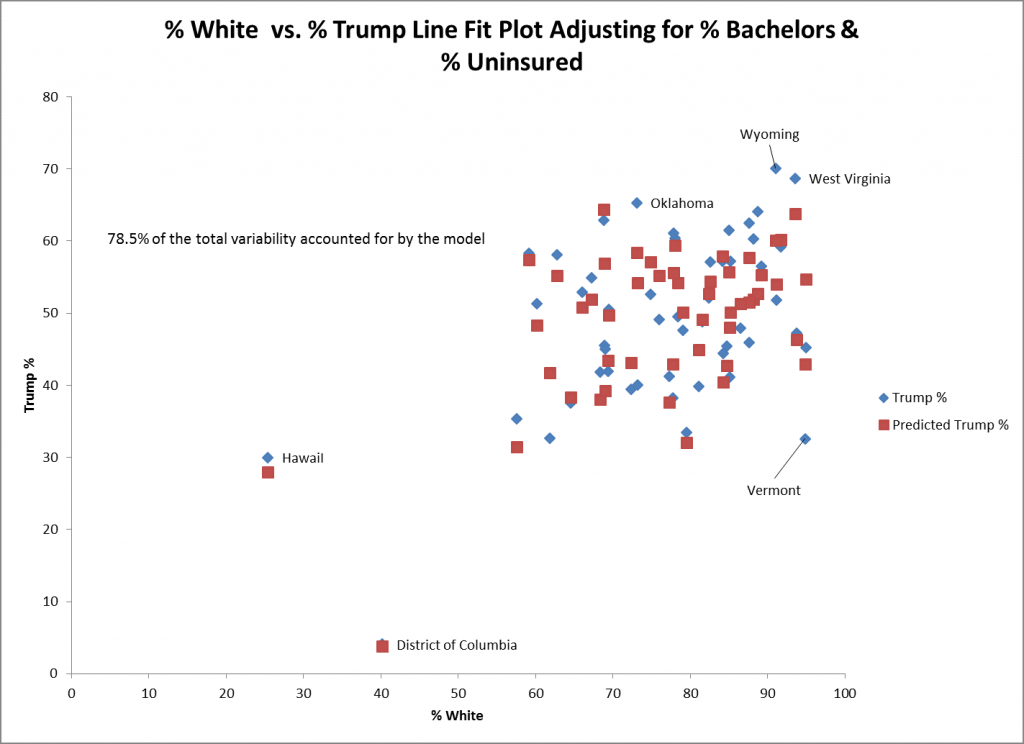
The scatterplot above shows the actual (in the blue diamond) and predicted values (in the red squares) for % white and % Trump for the model adjusting for % bachelors and % uninsured. The actual and predicted values for the District of Columbia (DC) and Hawaii are very close to each other which suggest good fit. One state that is poorly fit is Vermont where the actual vote for Trump is 10% lower than the predicted vote which can be seen directly above the blue diamond for Vermont.
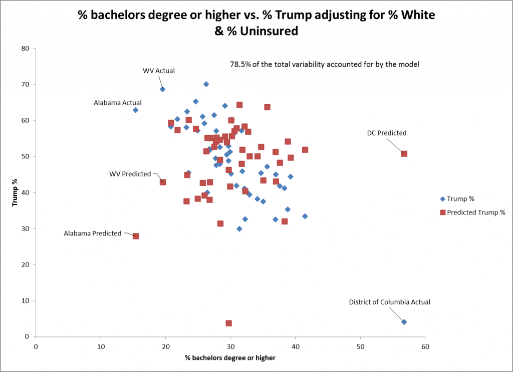
The scatter plot for % bachelor’s degree or higher suggests that the fit is not as good as it is for the one for % white as the predictor. This is reflected in the greater standard error for this predictor (0.15) than for % white (0.06). The prediction for DC is not as good for this predictor as it has the highest. The trend is still significant in the negative direction.
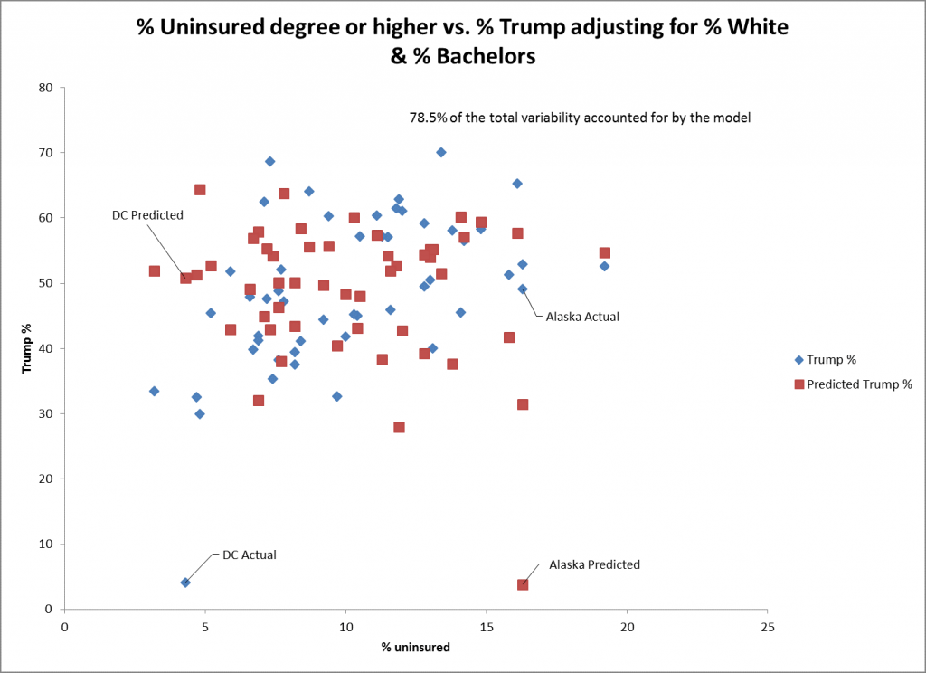
The scatterplot for % uninsured as a predictor shows even less fit for Trump’s % of the vote. DC and Alaska are poorly fit points for this predictor among many other states. The standard error for this predictor shows even less fit (0.26) for the other predictors though it’s still statistically significant.
Multiple regression is a potentially powerful tool for teasing apart the relationships between predictor variables for a specific outcome when conducted correctly. Adding the right covariates such as race can help alleviate the effects of an outlier such as Washington, DC. It’s always better to include all of the data to give the most complete picture of it as possible.
We now see that as the as the % of the population of a state with a bachelor’s degree or higher increases the % of the vote for Trump decreases. As at the same time, as the percentages of the white and uninsured in a state, increase the % of Trump’s vote increases. In the presence of these variables the concentration of hate groups and the % of the state in poverty are no longer significant predictors of Trump’s vote.
As Trump and the Republican controlled congress prepare to repeal the Affordable Care Act (ACA or as the GOP says Obamacare), the Congressional Budget Office estimates that 23 million Americans will lose their health insurance in the House version of the bill and an estimated 22 million will lose it in the Senate version. In this model the uninsured rate in each state is positively correlated with Trump’s vote. Does Trump believe that increasing the uninsured rate will increase their share of the vote in 2020?
Poverty was not associated with Trump’s vote in 2016. The decrease in uninsured estimates since the ACA went into effect in 2014 is mostly due to Medicaid expansion for the poorest individuals and subsidies which allow lower income individuals to purchase health insurance. Increasing the number of uninsured may not decrease Trump’s vote but it is unlikely to increase it.
Kolabtree helps businesses worldwide hire freelance scientists and industry experts on demand. Our freelancers have helped companies publish research papers, develop products, analyze data, and more. It only takes a minute to tell us what you need done and get quotes from experts for free.

Unlock Corporate Benefits
• Secure Payment Assistance
• Onboarding Support
• Dedicated Account Manager
Sign up with your professional email to avail special advances offered against purchase orders, seamless multi-channel payments, and extended support for agreements.


